Dates and Times with pandas.DatetimeIndex

Introduction
When working with data, one task that we might have to deal with often is manipulation of dates and times. The format provided in the dataset may not always be one which we can easily use in the various tasks required. Transforming from that format into one that can be easily used is something that forms a core part of the preparatory work needed to be performed on a dataset.
In this article, we shall explore the use of the Pandas function DatetimeIndex in transforming date data into a format we can use for further exploration.
We shall then look at a practical example using data from the Kiva for Good dataset.
Finally we shall use Streamlit to generate a dashboard from the practical examples.
Preliminary steps
Read in the Data
Import Pandas and read in the data. We shall use the kiva loans dataset. We shall use just the funded_amount and funded_time columns for this exercise.
| import pandas as pd | |
| df = pd.read_csv("data/kiva_loans.csv", usecols=[1,13]) | |
| df.dropna(inplace=True) | |
| df.reset_index(drop=True,inplace=True) | |
| df = df[["funded_amount", "funded_time"]] |

Conversion to datetime Object
Say you want to parse the funded_time column and get the different portions of the date (second, minute, hour, day, month, year). You could use regular text processing to do this (similar to the methods described in this article). Or you could use the Pandas DatetimeIndex function, which is what we shall use in this article.
If you explore the data types of the two columns, you will find that the funded_time column has the object data type.

First we need to convert the values in that column into a datetime object. For that we use the pandas.to_datetime() method.
| df["funded_time"] = pd.to_datetime(df["funded_time"]) |
When you now check the data types after performing this operation, you will see that the funded_time column is now of type datetime64[ns, UTC]. The number 64 indicates that the data is stored as a 64-bit integer. The ns indicates that this data is stored in units of nanoseconds. UTC indicates that this time is stored as Coordinated Universal Time (more on UTC can be found at the Bureau International des Poids et Mesures).

We can now proceed to process this column using the DatetimeIndex.
DatetimeIndex Methods and Attributes
Before processing all the rows, let us first pick out one instance of a timestamp and use that to walk through the various methods (denoted by parenthesis () after the name) and attributes.

Date
date() returns just the date portion of the time stamp.

Year
year returns the year.
is_year_start tests to see if it is the first day of the year.
is_year_end tests to see if it is the last day of the year.
is_leap_year tests to see if it is a leap year.

Quarter
quarter returns the quarter number of the year.
is_quarter_start tests to see if it is the first day of the quarter.
is_quarter_end tests to see if it is the last day of the quarter.

Month
month returns the month number.
month_name() returns the name of the month.
is_month_start tests to see if it is the first day of the month.
is_month_end tests to see if it is the last day of the month.

Day
day returns the date in the month.
day_name() returns the name of the day.
dayofweek returns the ordinal position of the day in a week. Monday is considered the first, with an ordinal position of 0.
dayofyear returns the number of the day in the year.
daysinmonth returns the number of days in that month.

Time
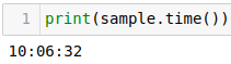
time() returns just the time portion of the time stamp.
Hour
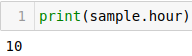
hour returns the hour of the day.
Minute
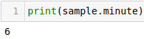
minute returns the minute of the hour.
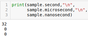
Second and Sub-Seconds
second returns the second of the minute.
microsecond returns microseconds.
nanosecond returns nanoseconds.
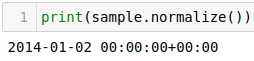
Normalize
normalize() this converts all times to midnight. It is useful in cases where the time does not matter, and all you are interested in is the date.
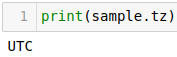
Timezones
tz returns the timezone of the timestamp.
tz_convert() converts the timestamp into one of the specified timezone. Provide the new timezone as Continent/City

Practical Example
Now that we have seen some of the attributes and methods of DatetimeIndex, let us use some of them in exploring our data. In this part, we shall answer a series of questions.
But before we get to the questions, we need to first set the index of our dataframe to the funded_time column. This will make it easier to get the required date or time component.
| df.set_index("funded_time",inplace=True) |

Without doing this, we would have to use a for loop or function to make the required change in an entire column as shown in the code snippet below:
| df["year"] = df["funded_time"].apply(lambda x: x.year) |
With the funded_time column set as the index, all we need to do is call the appropriate attribute or method to get the required change as shown below:
| df["year"] = df.index.year |
On to the questions.
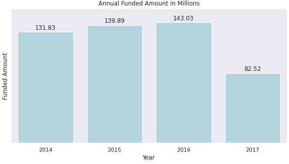
Question 1: What year saw the highest funded loan amounts?
Create a new column with years derived from the timestamp.
Aggregate funded amounts in each year.
Generate and display a dataframe with this information
| df["year"] = df.index.year | |
| year_aggregates = df.groupby("year")["funded_amount"].sum().sort_values(ascending=False).reset_index() | |
| year_aggregates |
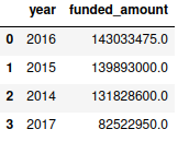
The resulting dataframe shows 2016 as having the highest funded amount. This is also visually evident from the Seaborn bar plot.
Question 2: In each year, which month recorded the highest funded amount?
Create a new column that has the month.
For each year, aggregate by month.
Identify the month with the highest funded amount.
Generate and display a dataframe that has year, month and funded amount.
| df["month"] = df.index.month_name() | |
| high_month_list = [] | |
| for year in list(df["year"].unique()): | |
| df_high_month = df[df["year"] == year][["year","funded_amount","month"]] | |
| df_high_month = df_high_month.groupby(["year","month"])["funded_amount"].sum().sort_values(ascending=False).head(1) | |
| high_month_list.append(df_high_month) | |
| df_high_month = pd.concat(high_month_list).reset_index() | |
| df_high_month |

We see that in each year other than 2017, December was the month that recorded the highest funded amount.
Question 3: Is there a specific day in each month that recorded the highest funded amount?
Create two new columns, one for number of month, and the second for day. The number of month column will be used to sort the final dataframe so that the months appear chronologically.
For each year, aggregate the daily funded amounts.
Get the day in each month that has the highest funded amount.
Generate and display a dataframe that has year, month, day and funded amount.
| df["month_number"] = df.index.month | |
| df["day"] = df.index.day | |
| high_day_list = [] | |
| for year in list(df["year"].unique()): | |
| df_year = df.groupby(["year","month","month_number","day"])["funded_amount"].sum().reset_index() | |
| df_year = df_year[df_year["year"] == year][["year","month","day","funded_amount", "month_number"]] | |
| for month in list(df["month"].unique()): | |
| df_high_day = df_year[df_year["month"] == month] | |
| df_high_day = df_high_day[df_high_day["funded_amount"] == df_high_day["funded_amount"].max()] | |
| high_day_list.append(df_high_day) | |
| df_high_day = pd.concat(high_day_list).reset_index(drop=True) | |
| sorted_df_high_day = [] | |
| for year in list (df_high_day["year"].unique()): | |
| sorted_df_high_day.append(df_high_day[df_high_day["year"] == year].sort_values(by="month_number")) | |
| df_high_day = pd.concat(sorted_df_high_day).reset_index(drop=True).drop("month_number","columns") | |
| df_high_day |

Let’s use Plotly Express to visualize this data.

We can see from the plot the days in each year that saw the highest funded amount.
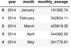
Question 4: For each month, what was the daily average funded amount?
Create a new column with number of days in month
Aggregate the funded amount per month for each year.
Get the average funded amount for each month.
Generate and display a dataframe with year, month and average funded amount.
| df["days_in_month"] = df.index.daysinmonth | |
| df_average = df.groupby(["year","month","month_number","days_in_month"])["funded_amount"].sum().reset_index() | |
| df_average["monthly_average"] = round(df_average["funded_amount"] / df_average["days_in_month"],2) | |
| sorted_df_average = [] | |
| for year in list(df_average["year"].unique()): | |
| sorted_df_average.append(df_average[df_average["year"] == year].sort_values(by="month_number")) | |
| df_average = pd.concat(sorted_df_average).reset_index(drop=True).\ | |
| drop(["month_number","days_in_month","funded_amount"],"columns") | |
| df_average |
An aside:
While going over the article before publishing, it occurred to me that I had not really checked to see if the daysinmonth attribute would report the correct number of days for February for leap years and regular years. At first I thought I would have to use the is_leap_year test in this portion of the exercise, but on further research I found that this has been well taken care of by DatetimeIndex.
To test this, I generated two dates in February, one on a leap year, one on a regular year, and checked the number of days in the month for both years. The expected results were produced by the code.

Like for the daily highest, let us visualize the monthly averages using a Plotly bar chart.

Going through these four examples should provide enough guidance on how to proceed. There’s more that can be gleamed from this data, and for that I leave it to you for further exploration.
Streamlit Dashboard
Finally, we can deploy a dashboard using Streamlit based on the brief exploration we have done. This will display a sample of the dataframe, plus the three plots generated in the course of this exercise.
For details on how to work with Streamlit, refer to this article.
Conclusion
In this article, we explored the methods and attributes of the Pandas function, DatetimeIndex.
We saw it’s use in extracting needed date and time information from a timestamp to aid in analysis of data.
We walked through several examples using sample data from the Kiva loans dataset.
Finally we deployed a dashboard showing a dataframe with the generated columns and some visualizations using Streamlit.
The Jupyter Notebook with the code from this article can be accessed here.
The Streamlit code for the dashboard deployment can be accessed here.